Rapid Multi-Objective Community Detection (RMOCD)

Availability
The Rapid Evolutionary Multi-objective Community Detection (re-mocd) algorithm is available as an open-source project on GitHub, where you can choose to compile it from source or use the precompiled library from releases. It is also available on Python’s PyPI, enabling seamless installation and usage. Today, in this publish date, the library has 48 files and 1,956 lines of code. The library supports two modes of operation: via the command-line interface (CLI) or through direct function calls using the PyPI library.
PyPI Usage
pip install re-mocd
For the Rust version, you will need to build it from the source code. Instructions for building can be found in the official repository. The run_rmocd function can be called as follows:
import re_mocd

partition = re_mocd.run("your.edgefile")
Given the graph below, the function produced the following partition:
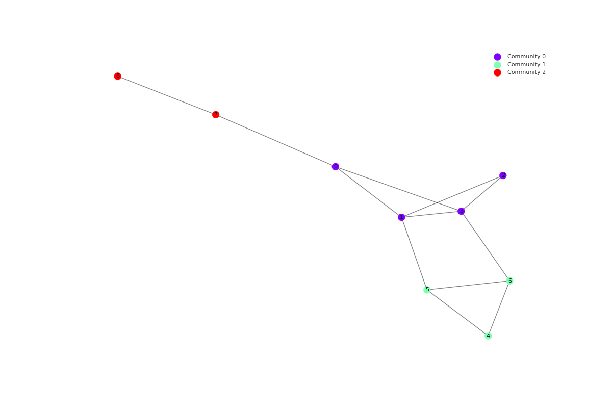
{0: 4, 1: 4, 2: 4, 3: 4, 4: 1, 5: 1, 6: 1, 7: 3, 8: 3}
In this representation, each entry corresponds to a node: community_id pair, indicating the community to which each node belongs.
Methodology
The primary goal of building this algorithm is to outperform the (Shi, 1) algorithm in terms of speed. Efficient handling of large graphs is crucial for many applications, making this a critical benchmark for success.
![Graphs used by the (Shi, [^shi]).](/publication/rmocd/Figures/graphs_shi2012.png)
Graphs used by the (Shi, [^shi]).
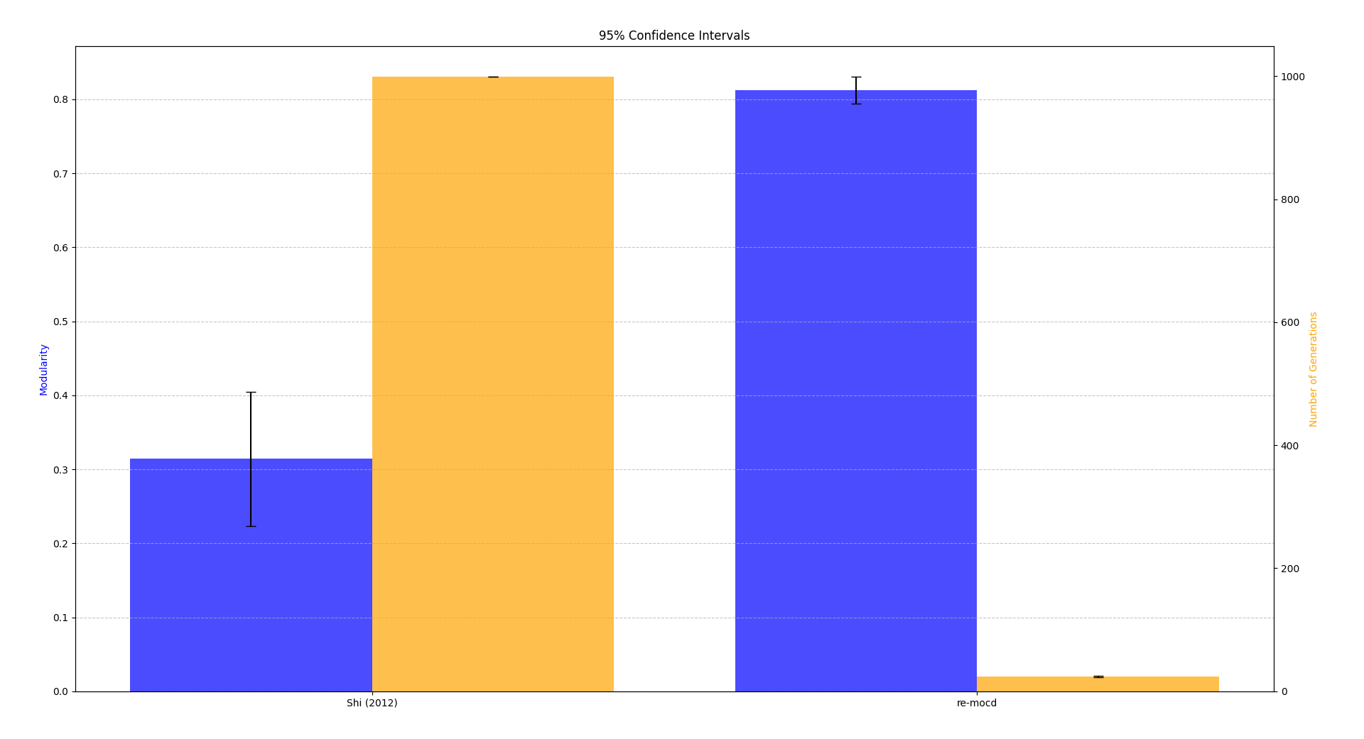
![Execution time comparison between the proposed algorithm (without PESA-II) and (Shi, [^shi]) (with PESA-II). The experiments were conducted on a machine with an 11th Gen Intel i5-11300H CPU (8 cores, 4.4 GHz) and 15,776 MB of RAM, with no GPU acceleration used.](/publication/rmocd/Figures/speed_comparison.png)
Execution time comparison between the proposed algorithm (without PESA-II) and (Shi, [^shi]) (with PESA-II). The experiments were conducted on a machine with an 11th Gen Intel i5-11300H CPU (8 cores, 4.4 GHz) and 15,776 MB of RAM, with no GPU acceleration used.
The (Shi, 1) algorithm does not provide the exact execution time for each dataset, only the average time per file. Using the same approach, the average execution time of the proposed algorithm across all files is 5.92 seconds, compared to 223 seconds. This demonstrates that the proposed algorithm is approximately 37.7 times faster.
Objective Function
The most computationally expensive part of the algorithm is the objective function, which corresponds to Equation (3.4) in (Shi, 1) paper:
$$ Q(C) = \sum_{c \in C} \left[ \frac{|E(c)|}{m} - \left( \frac{\sum_{v \in c} \text{deg}(v)}{2m} \right)^2 \right], $$where \(|E(c)|\) is the number of edges within community \(c\), \(m\) is the total number of edges, \(\text{deg}(v)\) is the degree of node \(v\), and \(C\) is the set of communities. The two terms reflect intra-community density and inter-community connectivity.
In our implementation, the corresponding computation complexity can be broken down as follows:
- Constructing the partition into communities involves iterating through all nodes and inserting them into a
HashMap. This operation scales as \(O(V)\), where \(V\) is the number of nodes. - For each community:
- Iterate through all nodes in the community.
- For each node, retrieve its precomputed degree (\(O(1)\)) and iterate through its neighbors. For each neighbor, a binary search checks membership in the community (\(O(\log |C|)\), where \(|C|\) is the size of the community).
- Since the degrees of the graph are precomputed once, the complexity for processing a single community is approximately: $$ O(|C| \cdot \log |C|), $$ removing the dependency on the degree \(d\).
- Aggregating results for \(k\) communities results in: $$ O(k \cdot |C| \cdot \log |C|) = O(V \cdot \log (V / k)). $$
Parallelization was achieved using par_iter() from the Rayon library, which distributes the workload of community processing across multiple threads. This reduces the effective workload per thread by a factor of \(p\), where \(p\) is the number of threads. The resulting complexity per thread is:
This significantly reduces computation time for large graphs.
Algorithm Complexity
Without PESA-II
In this approach, a pareto front is constructed from all genetic algorithm (GA) runs, followed by a selection of the maximum \(q\), where \(q\) represents the modularity of the objective function. Additionally, we parallelized the GA operators (selection, crossover, and mutation) using threads, represented by the parameter \(p\). As a result, the overall time complexity of the algorithm is:
$$ O\left( \frac{G \cdot P \cdot \left( V \cdot \log \left( \frac{V}{k} \right) \right)}{p} \right), $$where \(G\) is the number of generations, \(P\) is the population size, \(V\) is the number of nodes, and \(k\) is the average degree of the nodes.
PESA-II
In this case, we implemented the Pareto Envelope-based Selection Algorithm version 2 (PESA-II) in conjunction with parallelization of the GA operators (selection, crossover, and mutation) using threads. The resulting time complexity of the algorithm is:
$$ O\left( \frac{G \cdot P^2 \cdot \left( V \cdot \log \left( \frac{V}{k} \right) \right)}{p} \right), $$For comparison, the time complexity of the algorithm proposed by (Shi, 1) is:
$$ O(gs^2(m + n)). $$Genetic Operators: Enhanced Approaches
In genetic algorithms, initial generation, crossover and mutation are critical processes for combining and modifying candidate solutions. However, traditional approaches often fall short.
Limitations of Traditional Genetic Operators
Crossover Challenges
The crossover operation combines segments of two parent solutions to produce offspring. A commonly used method, the uniform two-point crossover, is described by (Shi, 1) as follows:
We choose the uniform two-point crossover because it is unbiased with respect to the ordering of genes and can generate any combination of alleles from the two parents.
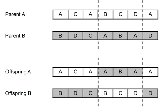
Example of how two-point crossover works
While versatile, this approach is problematic for community detection due to the following reasons:
- Lack of structural awareness: Crossover points are chosen without considering the graph’s partition or structural properties.
- Degradation of quality: The offspring often fail to preserve the characteristics of well-formed communities, leading to suboptimal solutions.
Mutation Challenges
Mutation introduces small random changes to solutions to maintain genetic diversity. In the traditional implementation, (Shi, 1) explains:
In the mutation operation, we randomly select some genes and assign them with other randomly selected adjacent nodes.
However, this approach has several drawbacks:
- Context-blind changes: It disregards the broader context of the solution, often disrupting the structural integrity of the partition.
- Random inefficiency: Mutations can lead to poorly constructed solutions, particularly when nodes critical to community structure are altered indiscriminately.
Initialization Challenges
The initial population sets the foundation for evolutionary progress. (Shi, 1) describes the traditional initialization process:
In the initialization process, we randomly generate individuals. For each individual, each gene \( g_i \) randomly takes one of the adjacent nodes of node \( i \).
Key issues include:
- Low-quality starting points: Random partitions are unlikely to reflect meaningful community structures.
- Search inefficiency: Starting too far from promising solutions hinders convergence in the vast search space.
Optimized Genetic Operators
1. Smart Crossover
- We ensures that the second point is never too close to the first, limiting the extent of the crossover and preventing drastic structural changes and preserves key community relationships ensuring that communities are not arbitrarily split or merged.
2. Smart Mutation
- A frequency cache is built to analyze community memberships among a node’s neighbors before deciding its assignment.
- After building the community frequency map for a node’s neighbors, the function selects the most frequent community.
- Nodes for mutation are selected based on a controlled mutation rate ($0.3$, different from the proposed $0.6$).
3. Smart Initialization
- The initial population is crafted to ensure diversity and better exploration:
- 33%: Random partitions for broad exploration.
- 33%: Neighbor-based partitions informed by graph structure.
- 34%: Special Cases
- 17%: Single community (all nodes in community \(\mu\))
- 17%: Based on node degree
| Strategy | Time Complexity |
|---|---|
| Random | O(PN log N) |
| Neighbor-based | O(P(N + E)log N) |
| Special Cases | O(P(N log N + E)) |
Results and Advantages
The tests were made 10 times for each strategy in a graph with 5000 nodes and 13712 edges.
We cleary see:
- Faster convergion and higher modularity
- Enhanced computational efficiency for large and complex graphs.
This happens because:
- Better preservation of community.
- More meaningful exploration of the solution space.
Tests
Info: The tests will not be conducted using the PyPI library. This decision is due to the performance limitations caused by Python’s Global Interpreter Lock (GIL). In simple terms, the GIL is a mutex (or lock) that restricts the Python interpreter to execute only one thread at a time, regardless of how many CPU cores are available. To avoid these limitations, we used a compiled version of the program and executed it via a Python subprocess, as shown below:
cmd = [mocd_path, graph_file]
if pesa_ii:
    cmd.append("--pesa-ii")
process = subprocess.run(cmd, check=True)
With Known Communities
To evaluate the performance of the algorithm, we chose the Louvain and Leiden algorithms for comparison. These community detection algorithms are widely recognized in academic research for their robustness and efficiency. To quantify the comparison, we utilized the Normalized Mutual Information (NMI) metric. NMI is a normalization of the Mutual Information (MI) score, which scales the results between 0 (indicating that there is no mutual information) and 1 (indicating perfect correlation).
The evaluation is structured as follows:
- Comparison using the algorithm without additional parameters.
- Comparison using the algorithm with the PESA-II implementation.
The tests were conducted using the following parameters to generate synthetic graphs with known communities:
size = 3~5
sizes = [10 * i for i in range(1, size+1)]
probs = [
    [0.5 if i == j else 0.1 for j in range(size)]
    for i in range(size)
]

G = networkx.generators.community.stochastic_block_model(
    sizes,
    probs,
    seed=42
)
- size: The number of communities in the graph. We will test 3 to 5 communities.
- sizes: A list specifying the number of nodes in each community, where community \(i\) contains \(10 \times i\) nodes.
- probs: A matrix defining the probabilities of connections within and between communities:
- Diagonal entries (\(i = j\)) represent the intra-community connection probability (set to 0.5).
- Off-diagonal entries (\(i \neq j\)) represent the inter-community connection probability (set to 0.1).
- G: The resulting graph generated using the stochastic block model with the specified sizes and probabilities. A fixed seed value of 42 ensures reproducibility.
Results
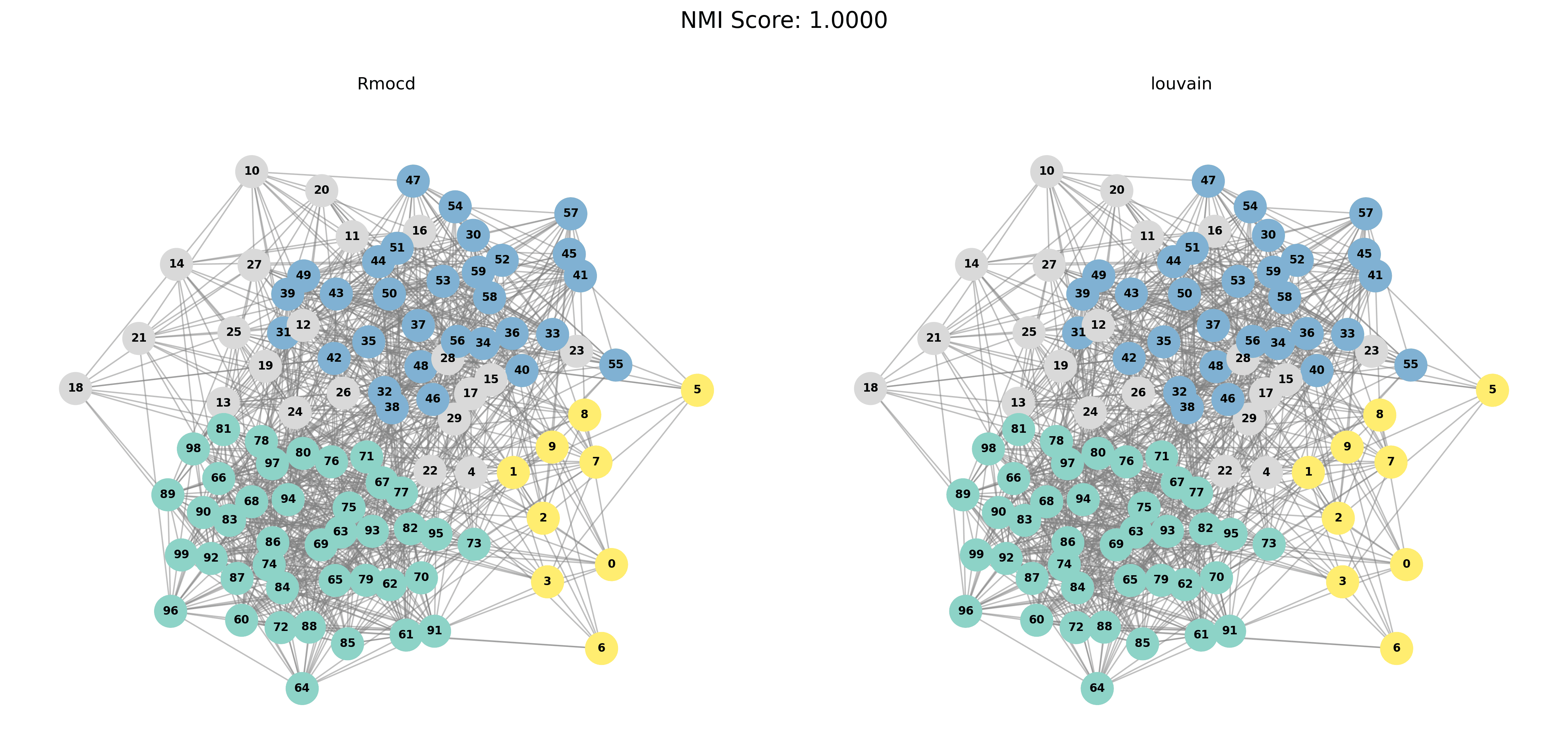
The results of the RMocd and RMocd PESA-II algorithms were compared for different graph sizes. For each size, the output of the algorithms is presented visually and evaluated using Normalized Mutual Information (NMI). Table 1 summarizes the performance metrics.
| Size | Algorithm | Iterations | Runtime (s) | NMI Louvain | NMI Leiden |
|---|---|---|---|---|---|
| 3 | RMocd | 149 | 1.09 | 1.00 | 0.27 |
| RMocd PESA-II | 168 | 2.73 | 0.63 | 0.21 | |
| 4 | RMocd | 211 | 1.43 | 1.00 | 0.09 |
| RMocd PESA-II | 278 | 3.82 | 0.61 | 0.21 | |
| 5 | RMocd | 413 | 1.92 | 0.95 | 0.07 |
| RMocd PESA-II | 513 | 6.53 | 0.35 | 0.24 |
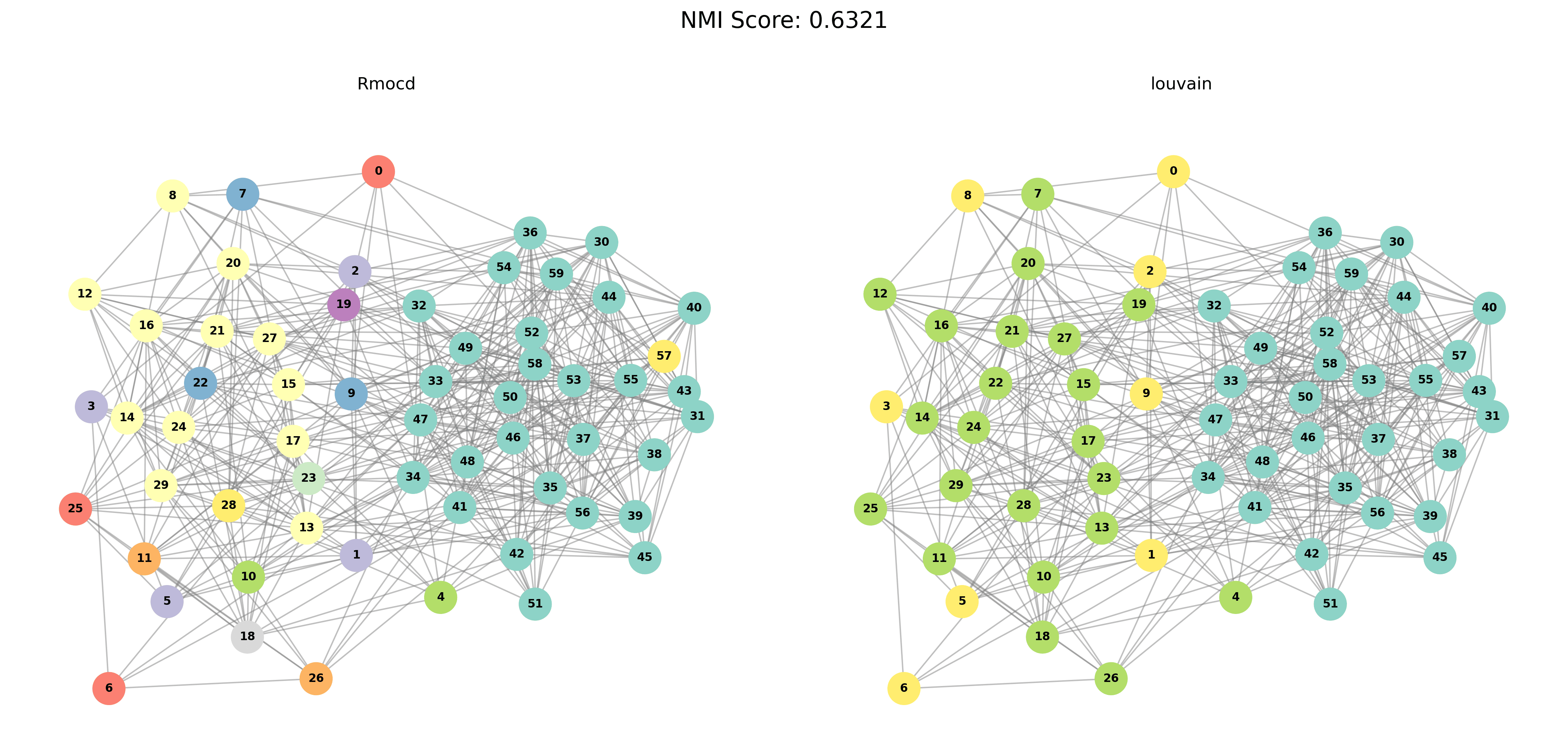
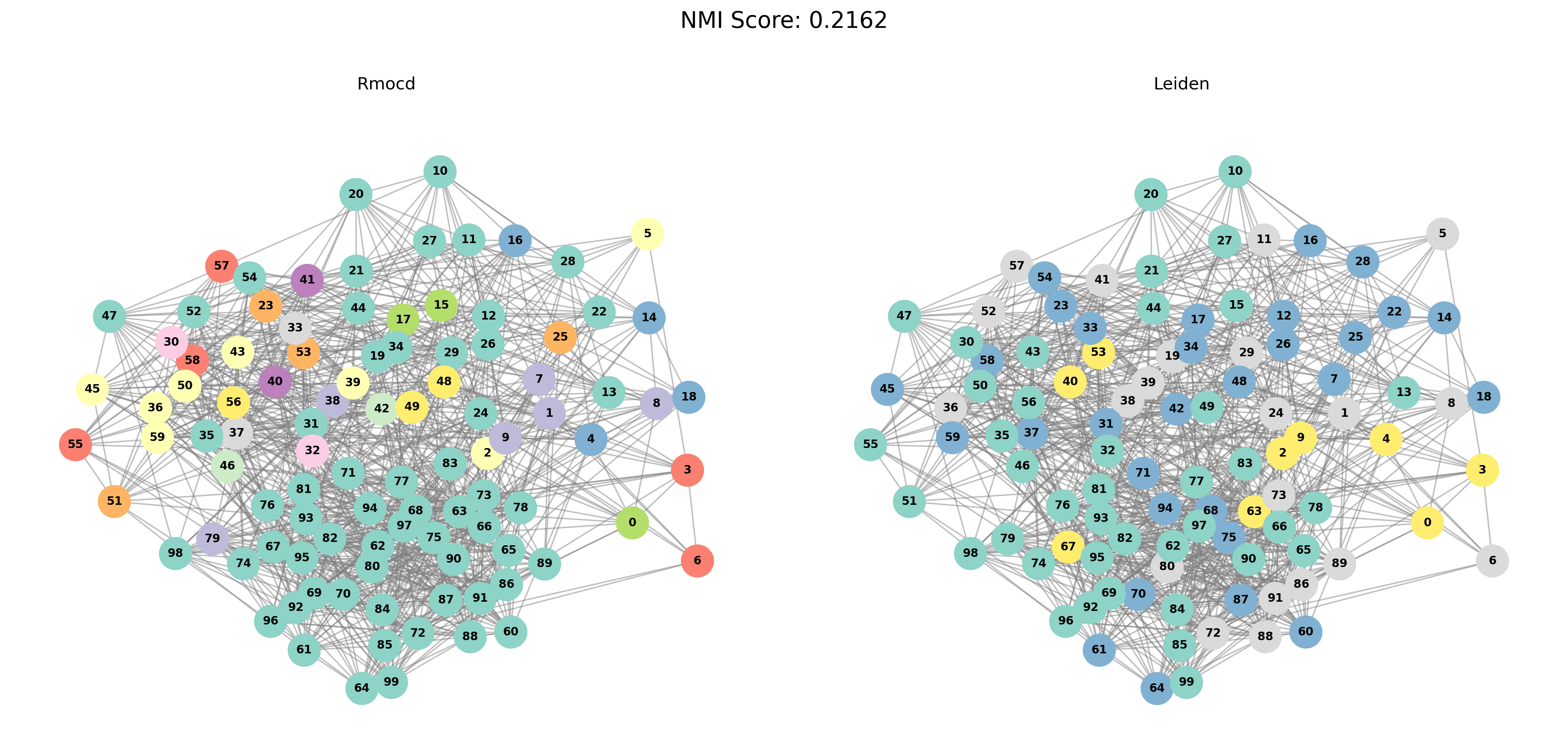
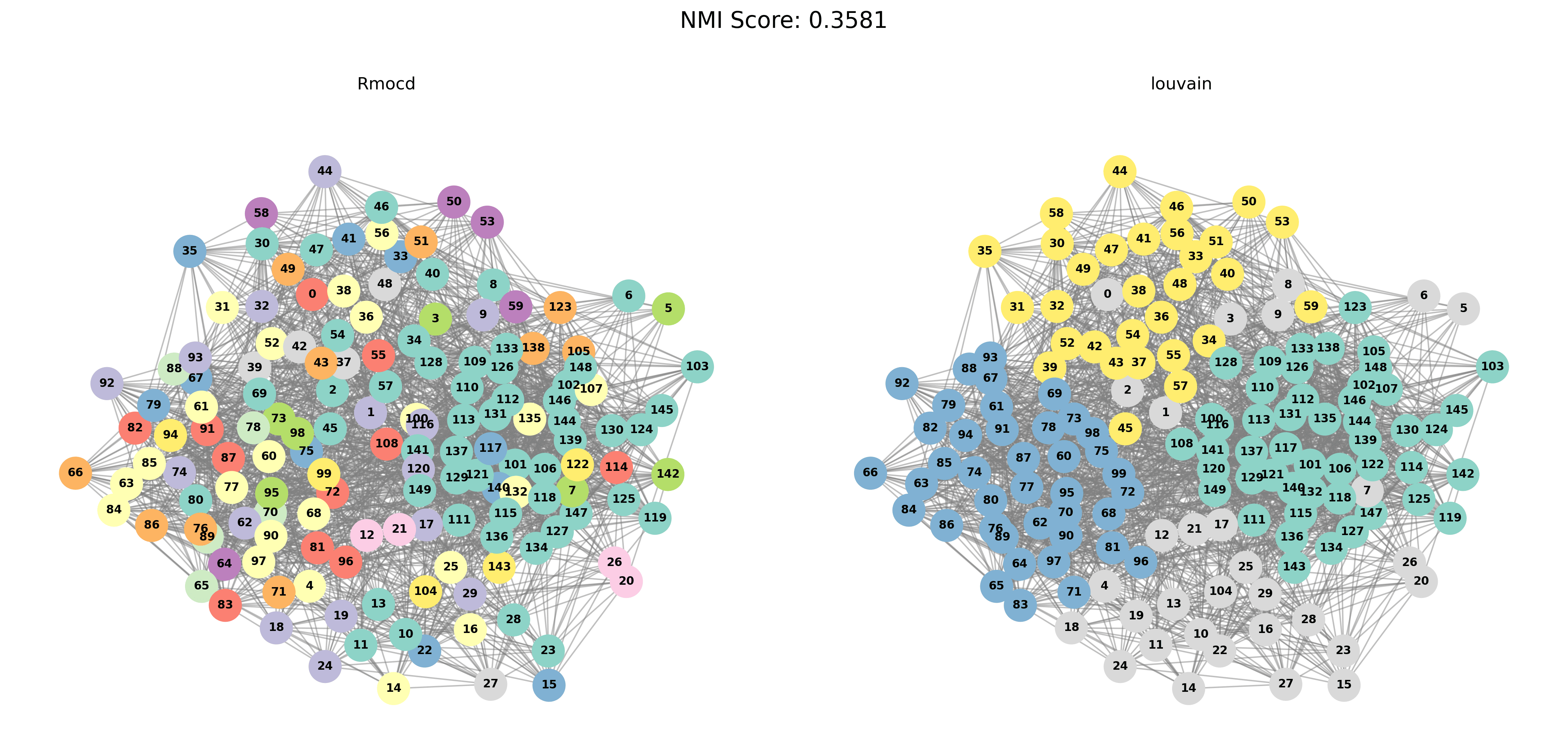
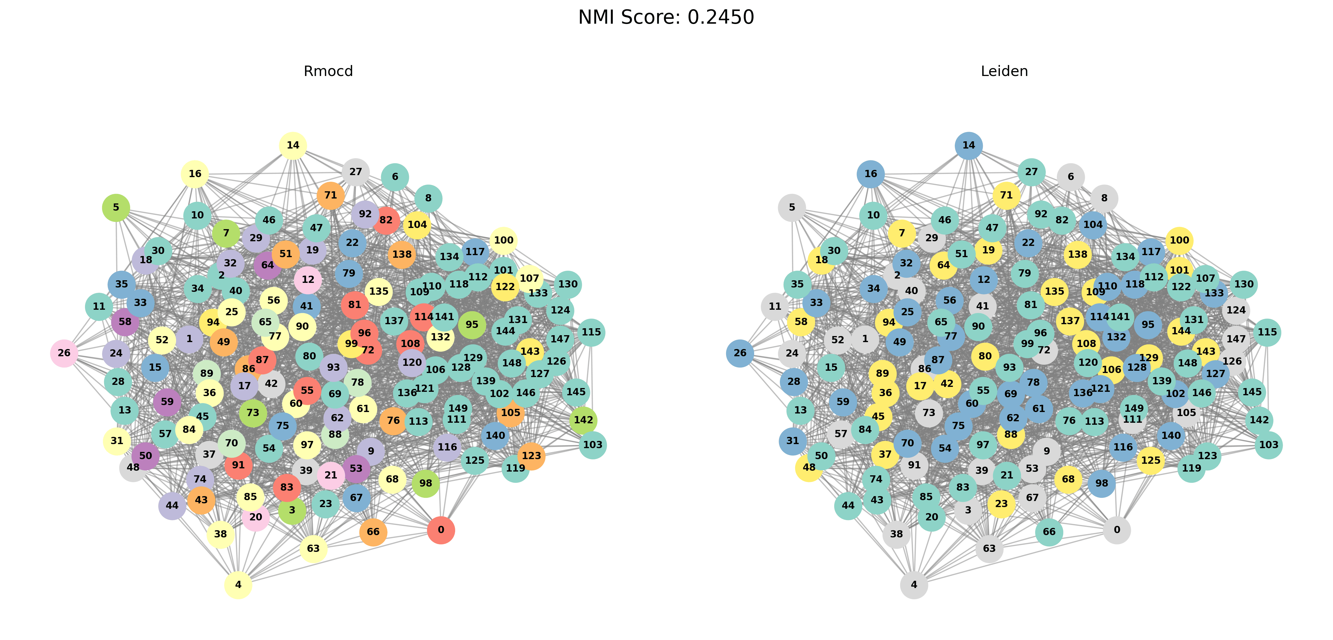
Visual Comparisons of Community Detection
To provide a visual representation of the community detection results, we present the output of the Louvain and Leiden algorithms for different graph sizes (3 to 5 communities). Each row in the sections below shows the comparison for a specific graph size, with Louvain’s results on the left and Leiden’s results on the right.
Without PESA-II
| Louvain Results | Leiden Results |
|---|---|
 | 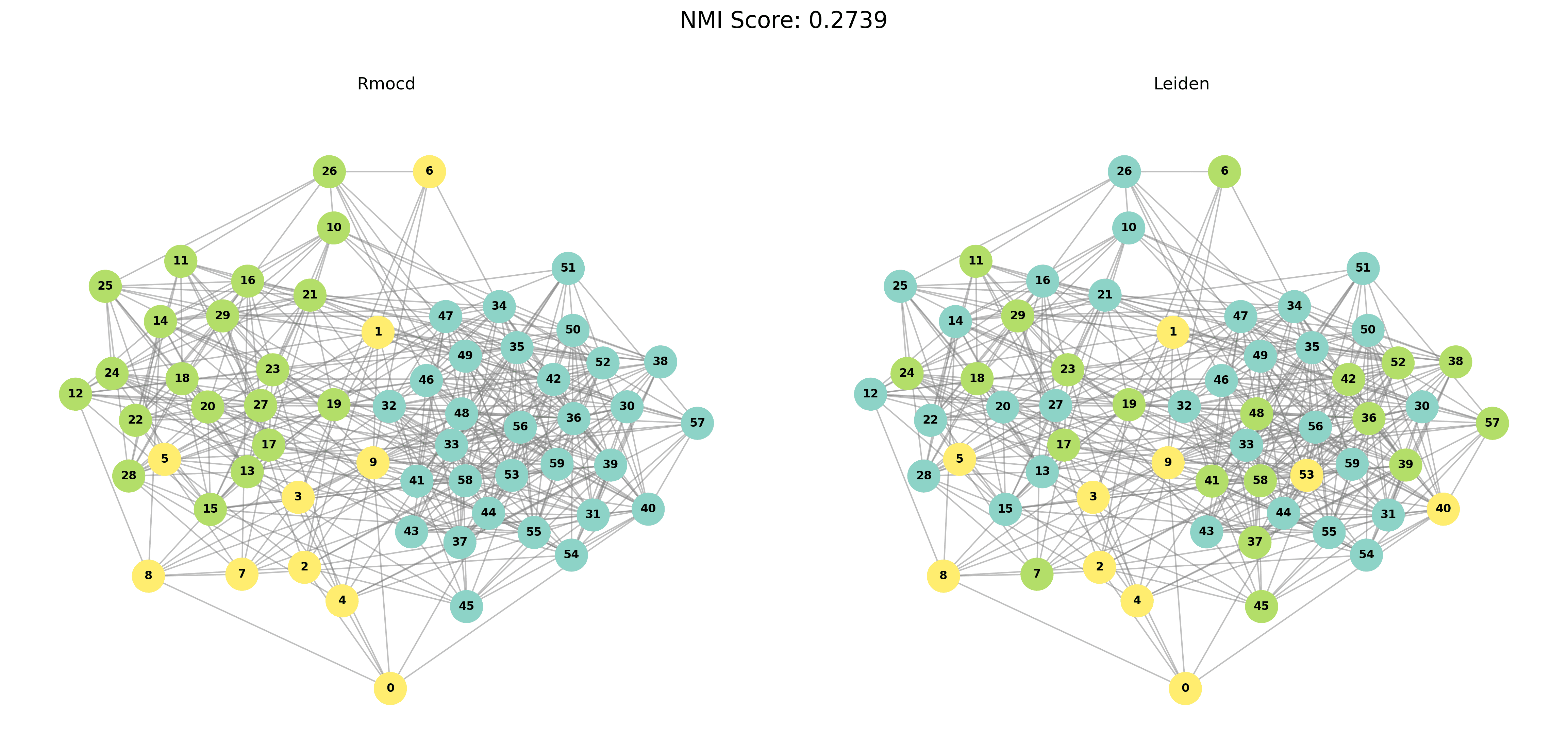 |
 | 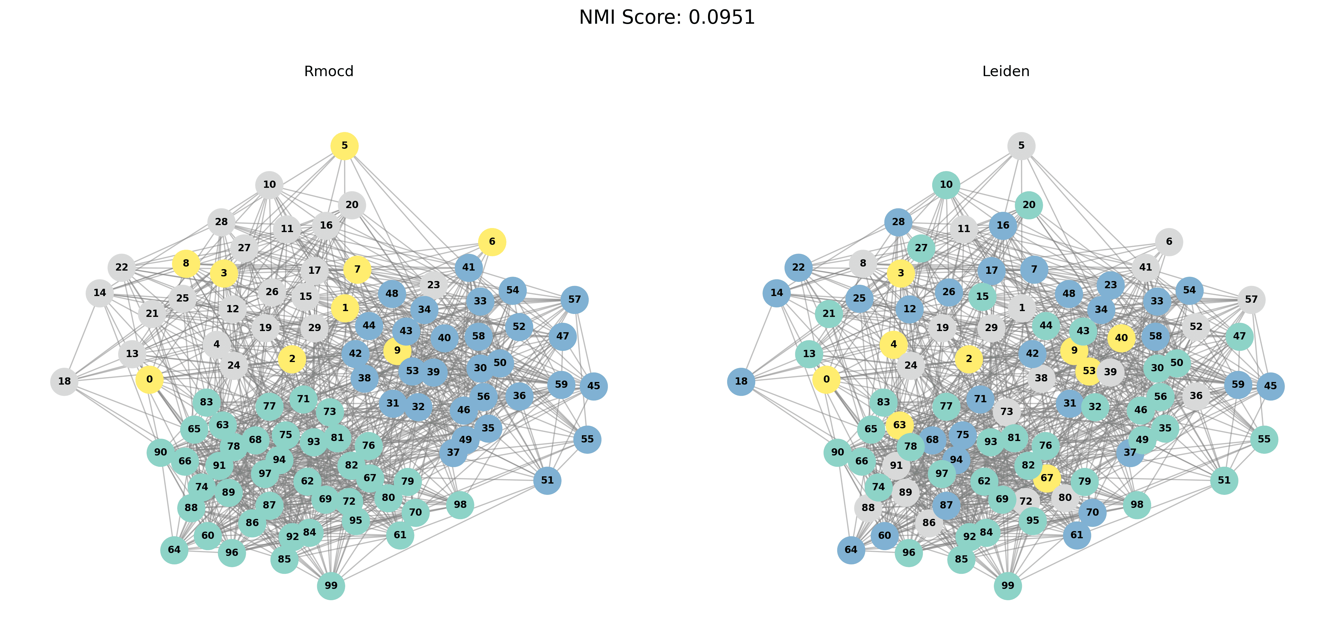 |
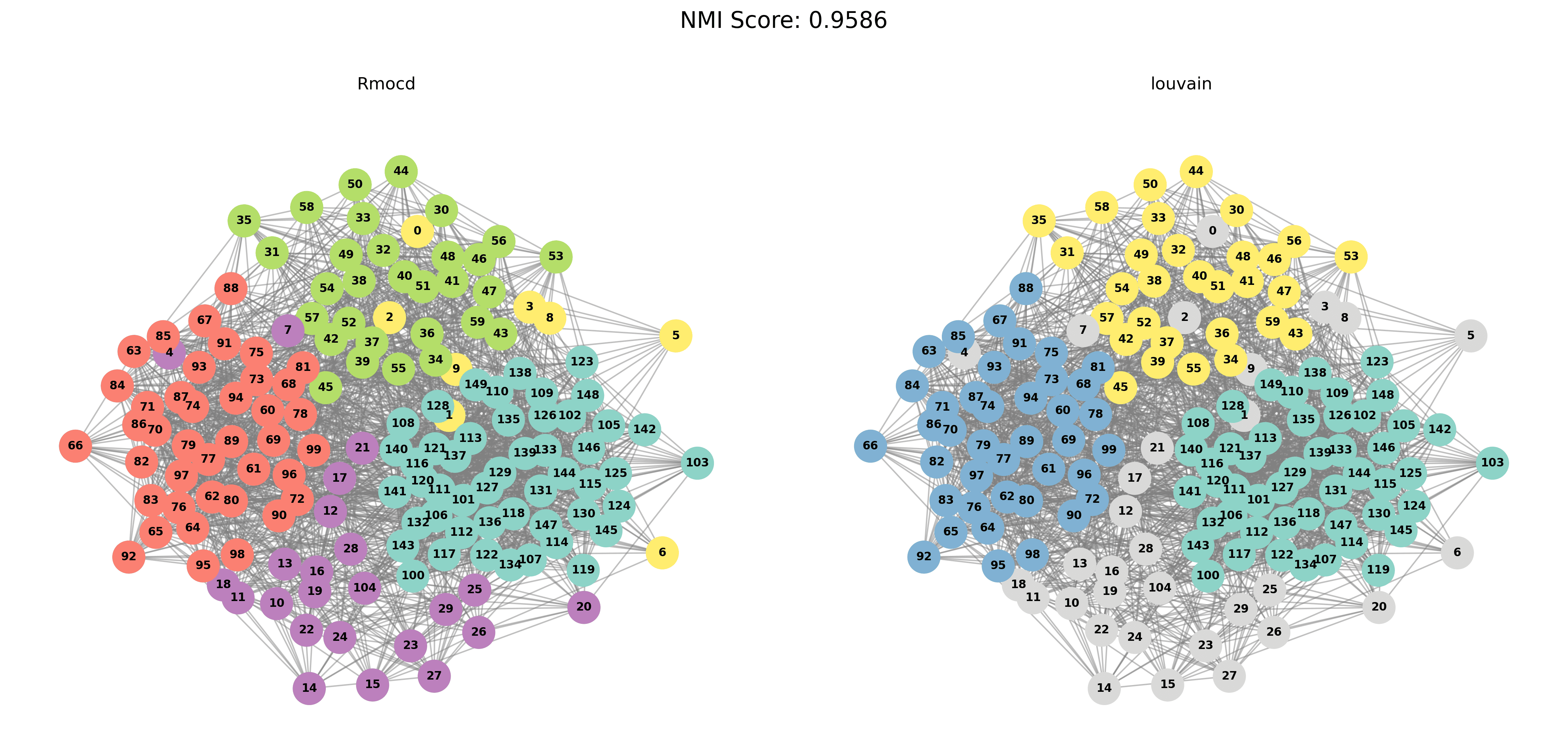 | 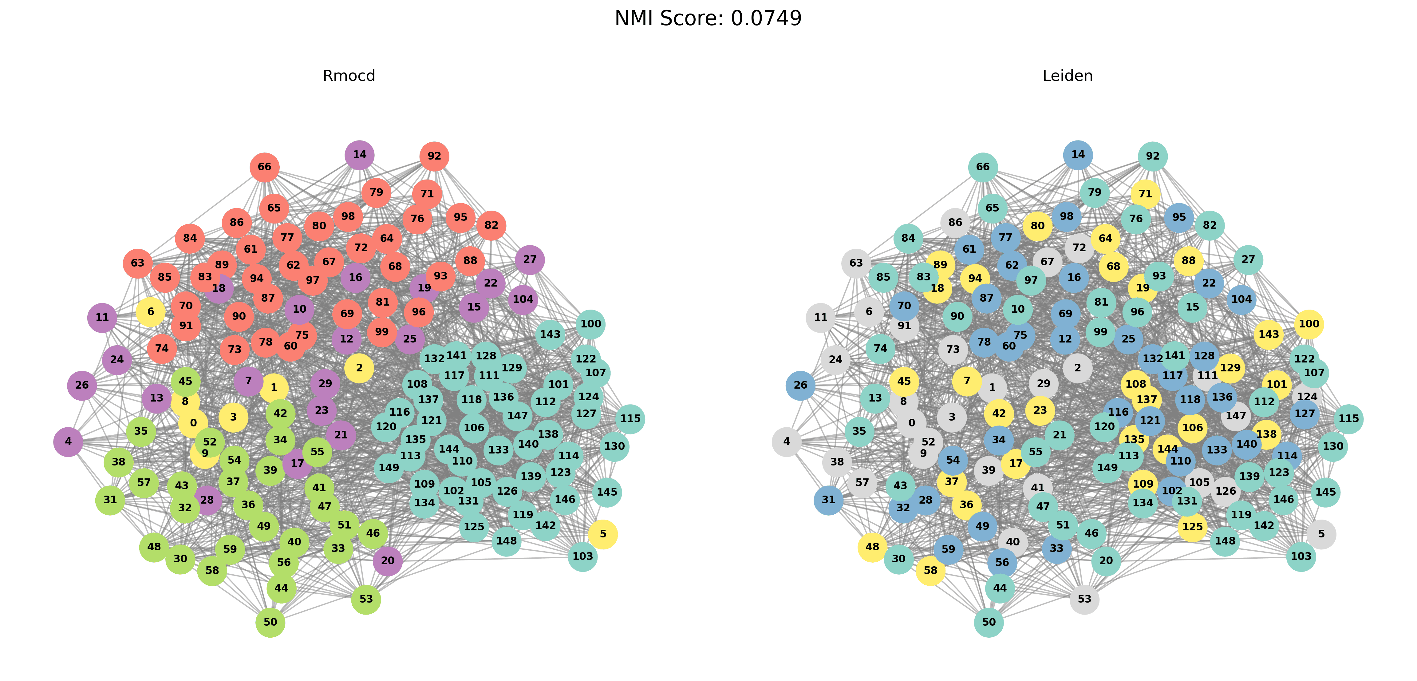 |
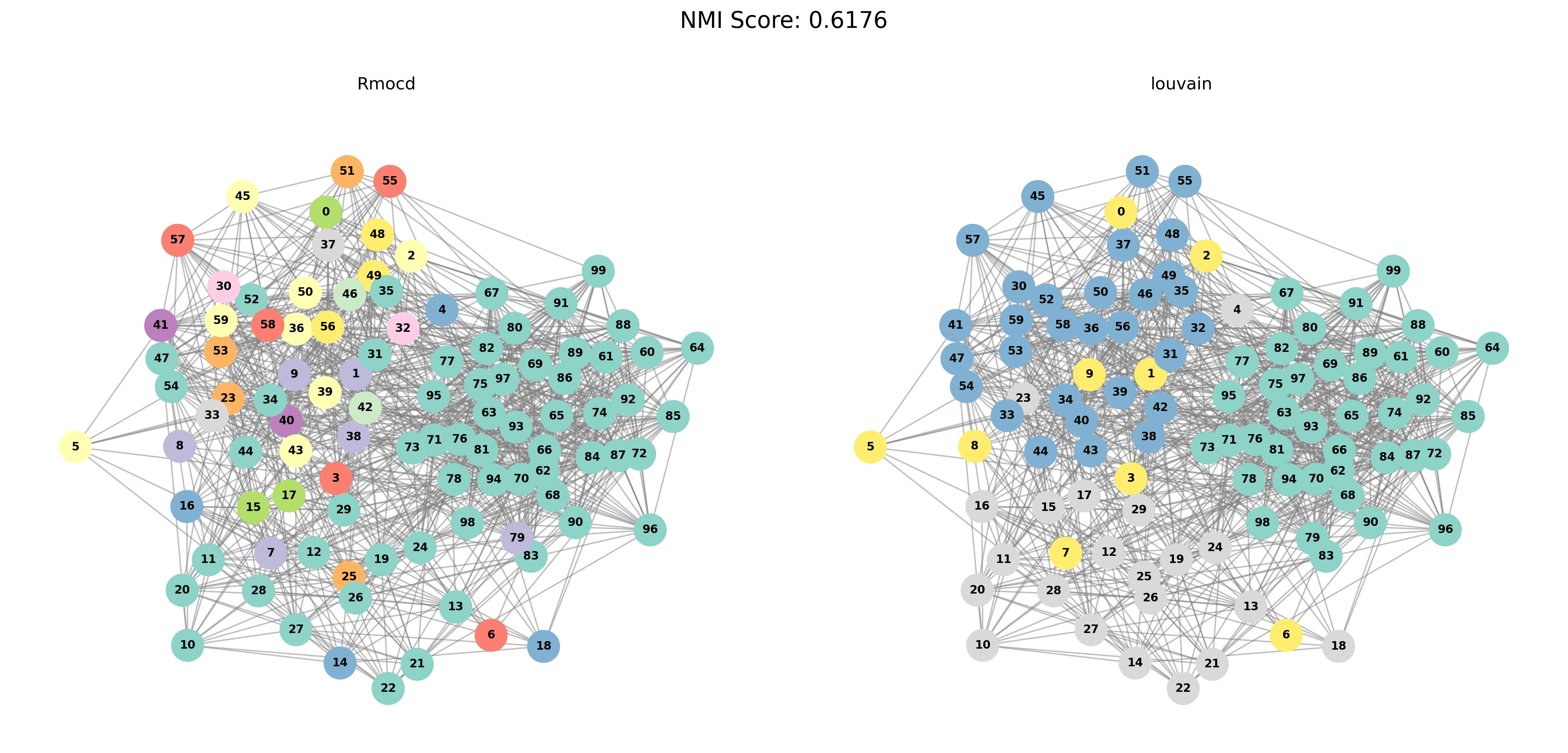
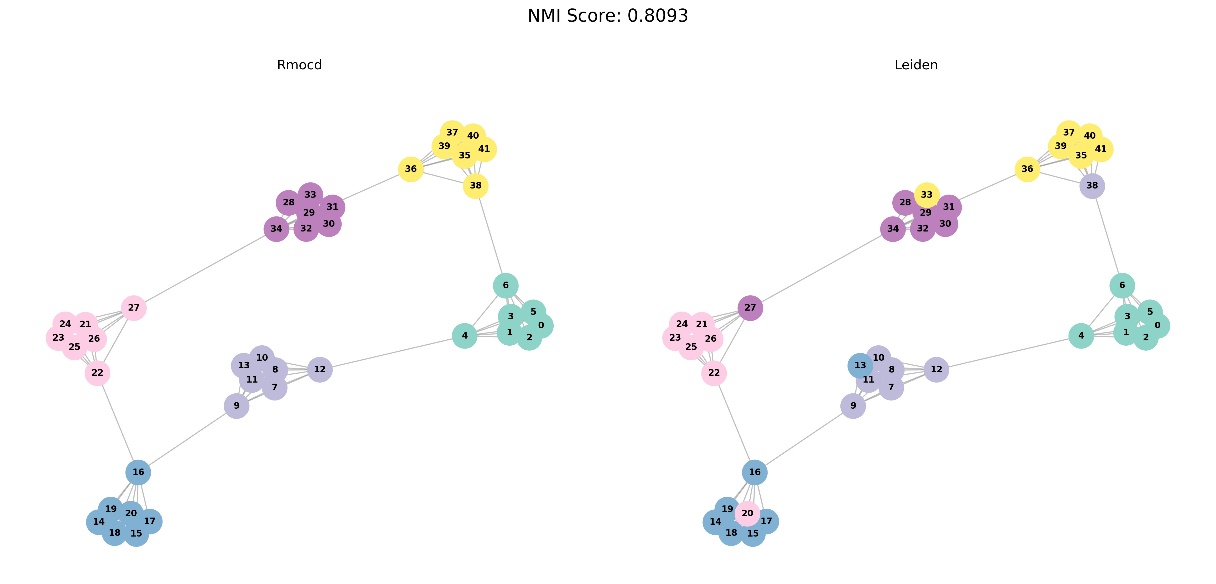
With PESA-II
| Louvain Results | Leiden Results |
|---|---|
 | 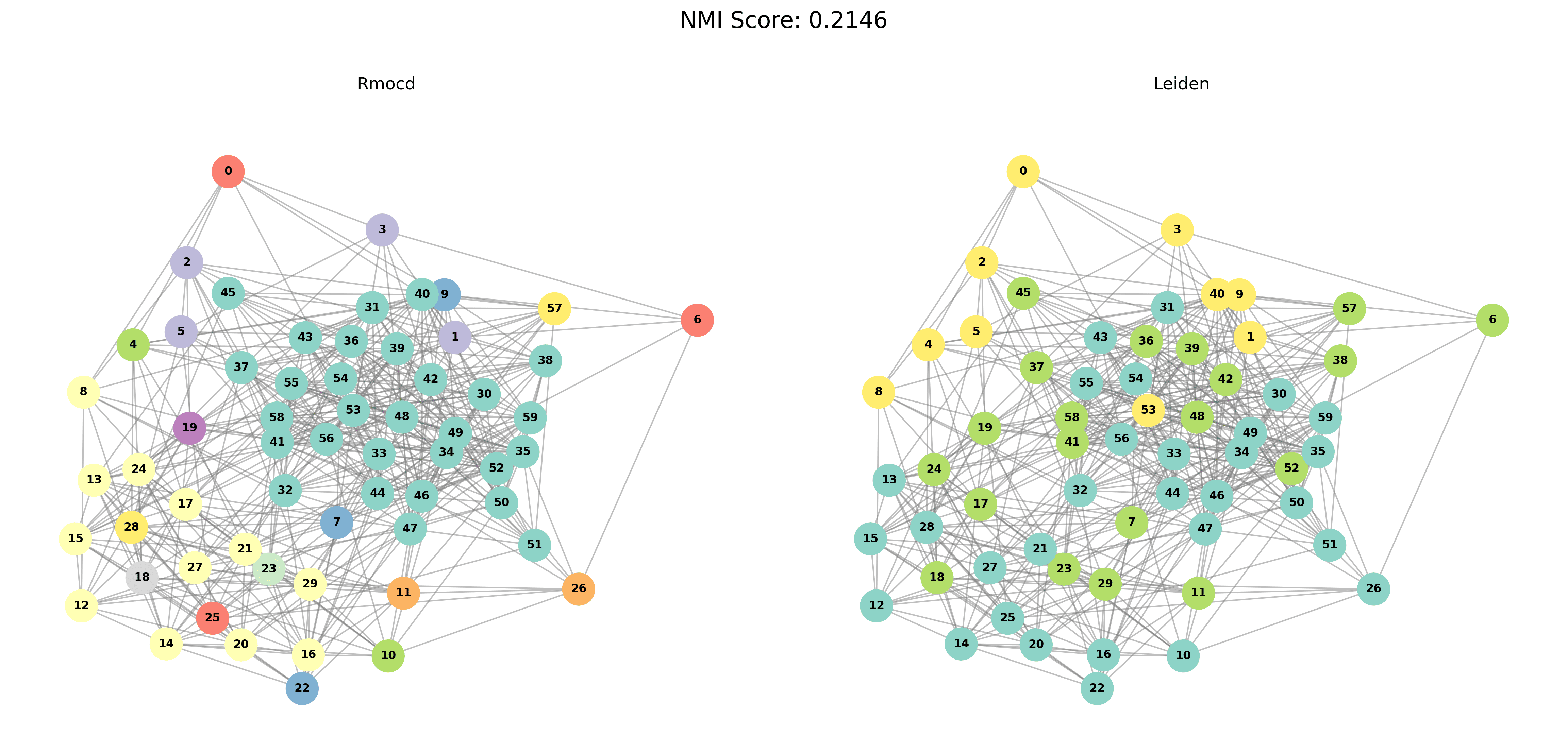 |
 |  |
 |  |
Based on \(\mu\) (mu)
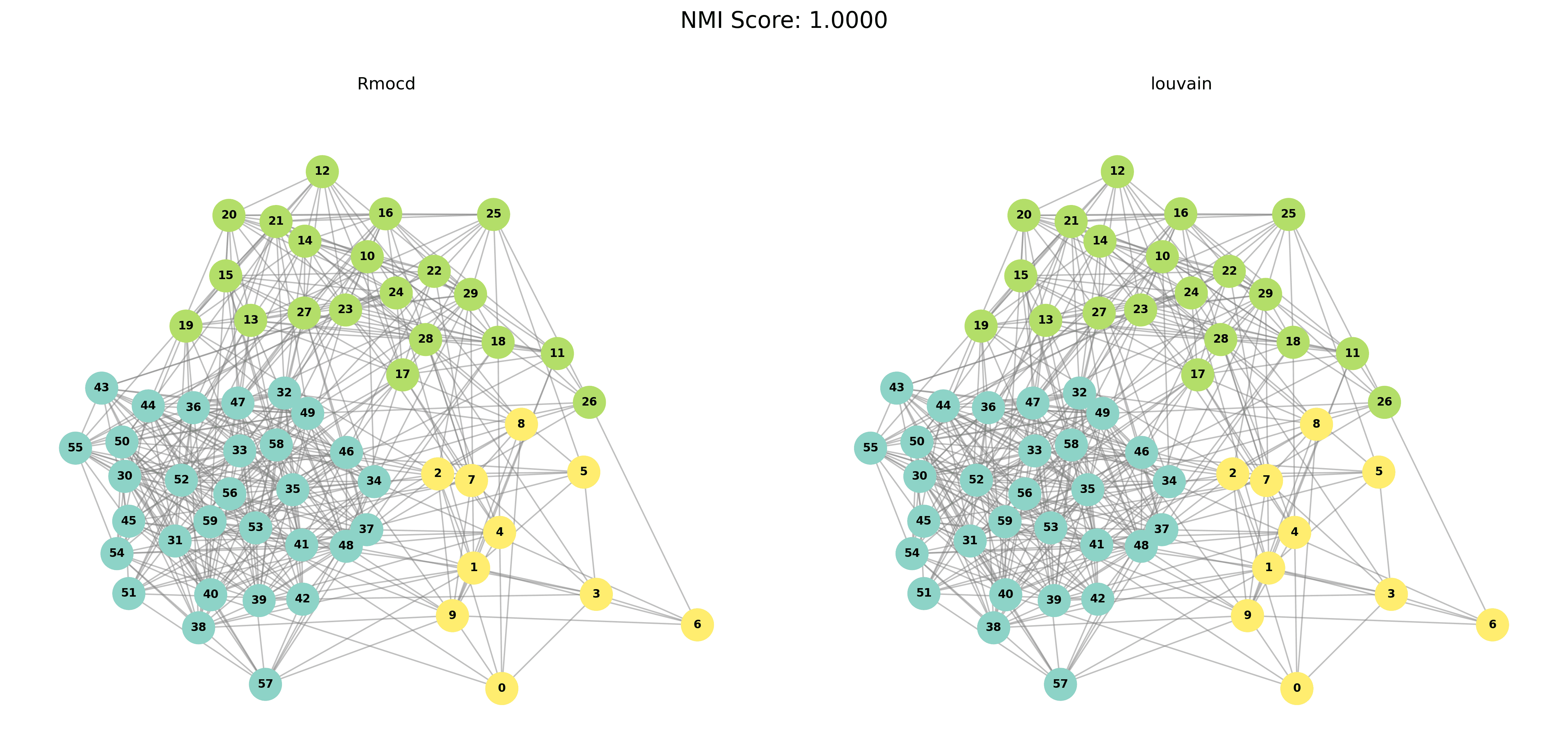
In this test, we use LFR benchmark graphs generated by the networkx Python library. Unlike the stochastic block model, the number of communities in the graph is not explicitly defined; instead, we only specify the maximum and minimum sizes of the communities. The \(\mu\) value represents the fraction of inter-community edges incident to each node and must lie within the interval \([0, 1]\). This parameter allows us to analyze the differences between Leiden and Louvain algorithms as the \(\mu\) value increases.
![Graphs used by the (Shi, [^shi])](/publication/rmocd/Figures/nmi.png)
Graphs used by the (Shi, [^shi])
Other Tests
RMocd addresses certain issues associated with modularity in other community detection algorithms. For example, in Figure 1, we illustrate a network consisting of a ring of cliques connected by single links. This scenario highlights the limitations of modularity-based methods in resolving community structures.
The network consists of cliques, each represented as a complete graph \(K_m\) with \(m\) nodes and \(m(m - 1)/2\) links. Assuming \(n\) cliques (with \(n\) being even), the network has a total of \(N = nm\) nodes and \(L = nm(m - 1)/2 + n\) links.
References
Chuan Shi a, Zhenyu Yan, Yanan Cai, Bin Wu. Multi-objective community detection in complex networks. Elsevier, Beijing University of Posts and Telecommunications, Beijing Key Laboratory of Intelligent Telecommunications Software and Multimedia, Beijing 100876, China. Research Department, Fair Isaac Corporation (FICO), San Rafael, CA 94903, USA. Available at: https://www.sciencedirect.com/ ↩︎ ↩︎ ↩︎ ↩︎ ↩︎ ↩︎ ↩︎